Creating Cool UI: SwiftUI Mesh Gradients, from Control Points to Metal
Building SwiftUI mesh gradients with UIKit, understanding their Bézier patches, and recreating the effect in UIKit and Metal with adaptive geometry
A mesh gradient lets me put colors at positions in two dimensions, then bend the transitions between them. A small change to a point can pull a bright region across the view, stretch a ribbon of color, or turn a regular grid into something that looks like moving liquid.
SwiftUI added MeshGradient in iOS 18 and macOS 15. I wanted the same kind of effect in UIKit, with ordinary mutable properties, UIKit animation blocks, and support for older iOS versions. That became KHMeshGradient: an independent UIKit view backed by Metal, targeting iOS 15 and later.
Before getting into the implementation, here is what the SwiftUI API can do:
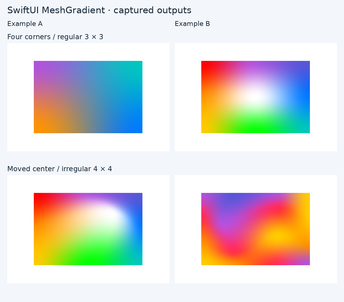
These are captured renders, not mockups. The first part of this article builds up those examples. Then I'll look at the mesh beneath the colors, translate that into Metal, and compare the output and performance of the two renderers.
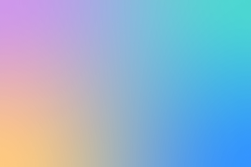
Start with four colors
The simplest useful mesh has two points across and two points down. Its four vertices define one patch:
import SwiftUI
import UIKit

@available(iOS 18.0, *)
struct FourCornerMesh: View {
	var body: some View {
		let colors: [Color] = [
			Color(Color.RGBColorSpace.sRGB, red: 0.686, green: 0.322, blue: 0.871),
			Color(Color.RGBColorSpace.sRGB, red: 0, green: 0.78, blue: 0.745),
			Color(Color.RGBColorSpace.sRGB, red: 1, green: 0.584, blue: 0),
			Color(Color.RGBColorSpace.sRGB, red: 0, green: 0.478, blue: 1)
		]
		MeshGradient(
			width: 2,
			height: 2,
			points: [
				[0, 0], [1, 0],
				[0, 1], [1, 1]
			],
			colors: colors,
			colorSpace: Gradient.ColorSpace.device
		)
		.frame(width: 360, height: 240)
	}
}
This first example is self-contained. The remaining snippets reuse MeshExamples, the palette/grid helper enum defined in the complete Swift examples. Its palettes are [UIColor], and its grids are [SIMD2<Float>]. SwiftUI view expressions below belong inside a View.body; import SwiftUI and UIKit. Using the same resolved sRGB colors matters for comparisons: a named SwiftUI color and a UIKit semantic color are not a reliable promise of identical values across systems and appearances.
The points are SIMD2<Float> values in normalized coordinates. (0, 0) is the top-left corner; (1, 1) is the bottom-right. Both arrays run left to right, row by row. The color at index 2 belongs to the position at index 2.
width and height describe the input grid, not the number of pixels or GPU triangles. A 2 × 2 input grid contains four colored vertices and one patch. A 3 × 3 grid contains nine colored vertices and four patches. In general:
patch count = (width - 1) × (height - 1)
Add a center, then move it
A 3 × 3 grid gives me a color in the middle and a position to move independently of the boundary:
let points: [SIMD2<Float>] = [
	[0, 0],   [0.5, 0],   [1, 0],
	[0, 0.5], [0.5, 0.5], [1, 0.5],
	[0, 1],   [0.5, 1],   [1, 1]
]

// Inside a SwiftUI view's body:
MeshGradient(
	width: 3,
	height: 3,
	points: points,
	colors: MeshExamples.rainbow.map({ (color: UIColor) -> Color in
		Color(uiColor: color)
	}),
	colorSpace: Gradient.ColorSpace.device
)
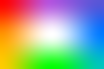
Now keep the colors unchanged and move the middle vertex:
var warped: [SIMD2<Float>] = points
warped[4] = SIMD2<Float>(0.72, 0.28)
Pass warped instead of points to the same initializer:
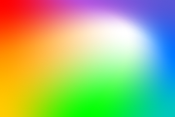
The white region moves, but so do the paths connecting its neighbors. This is why changing geometry produces a different effect from simply changing the center color. The mapping of the entire patch changes around it.
For an ordinary continuous design, keep the points in a sensible progression across rows and down columns. Crossing points or pulling handles far past one another can fold patches and introduce overlaps. That can be a deliberate effect, but it complicates coverage and matching another renderer.
A more organic 4 × 4 mesh
The next example has 16 colored vertices and nine patches. The irregular interior positions introduce curves without moving the outer boundary away from the view's edges:
let organicPoints: [SIMD2<Float>] = [
	[0, 0],   [0.3, 0],   [0.7, 0],   [1, 0],
	[0, 0.3], [0.2, 0.4], [0.7, 0.2], [1, 0.3],
	[0, 0.7], [0.3, 0.8], [0.7, 0.6], [1, 0.7],
	[0, 1],   [0.3, 1],   [0.7, 1],   [1, 1]
]

MeshGradient(
	width: 4,
	height: 4,
	points: organicPoints,
	colors: MeshExamples.organicColors.map({ (color: UIColor) -> Color in
		Color(uiColor: color)
	}),
	colorSpace: Gradient.ColorSpace.device
)

Mesh gradients in SwiftUI by Natalia Panferova is a useful introduction to the API and inspired these example fixtures. The downloadable examples contain the full palettes, including the resolved colors used for our comparisons.
Smoothing, transparency, and uncovered space
Geometry is only part of the effect. smoothsColors controls how colors transition across the patches. The default smooth interpolation derives cubic curves from neighboring colors. Setting it to false gives linear color transitions in the patch coordinates; it does not turn the curved geometry into straight edges.
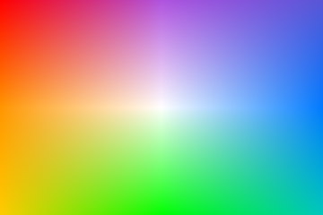
If the bottom-right point moves inward to [0.8, 0.9], the mesh stops covering part of the view. SwiftUI's background: parameter fills that uncovered region:
MeshGradient(
	width: 2,
	height: 2,
	points: [[0, 0], [1, 0], [0, 1], [0.8, 0.9]],
	colors: MeshExamples.corners.map({ (color: UIColor) -> Color in
		Color(uiColor: color)
	}),
	background: Color(uiColor: MeshExamples.indigo),
	colorSpace: Gradient.ColorSpace.device
)
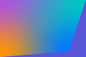
That fill is distinct from the view behind a translucent mesh. Reducing a vertex's alpha reveals the underlying view through the mesh; the mesh's own outside-fill color does not become a backing plate beneath those translucent pixels.
What is the mesh actually doing?
The visible colors can make the effect look like several blurred circles. The underlying representation is a collection of connected, curved patches.
Here are our Metal renders with the library's debug overlay beside them. The overlays are produced by our renderer, not captured from a SwiftUI debugging API:
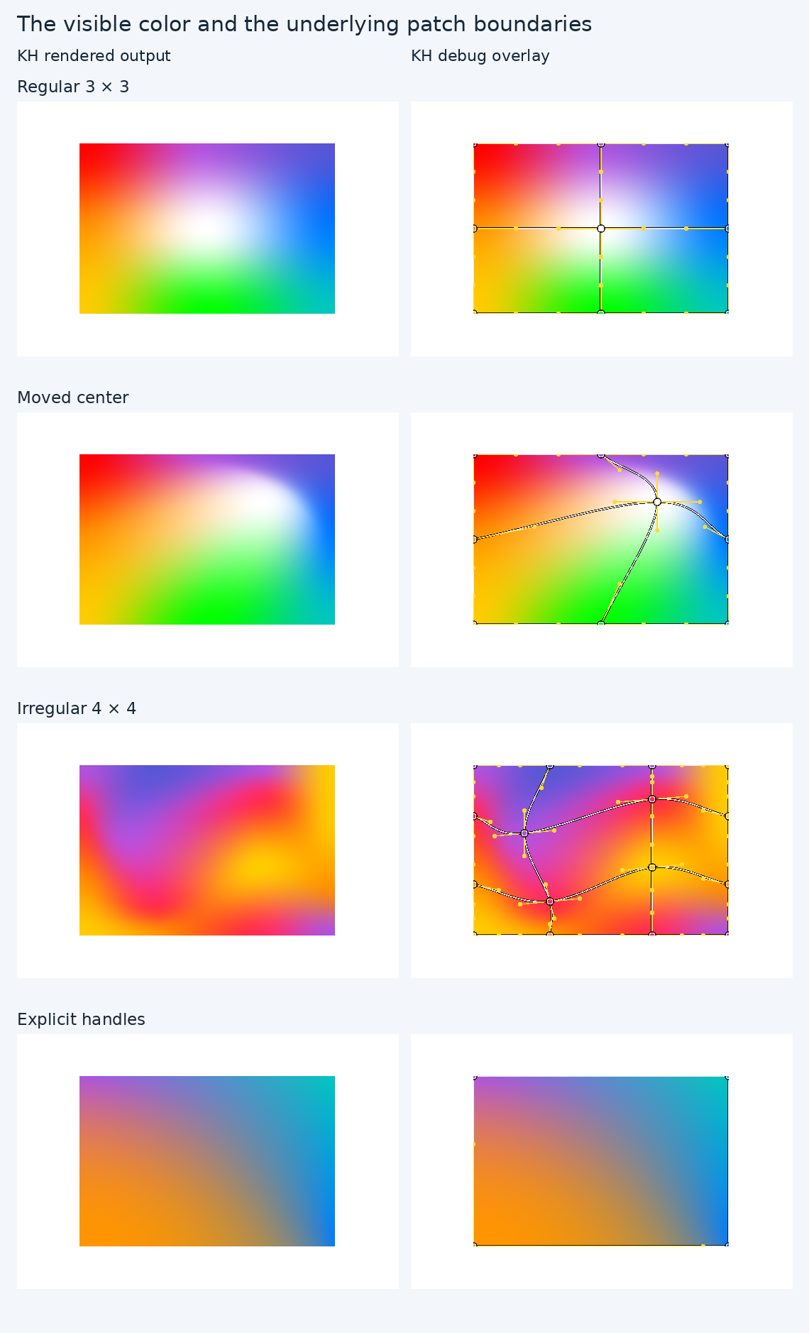
The main dots are the colored input vertices. The lines joining them are patch boundaries. In the explicit-handle example, the additional handle lines show how the boundary tangents are controlled. Debug overlays are drawn on top of the gradient; they are not part of the color calculation.
Each SwiftUI MeshGradient.BezierPoint has a position and four handles: leading, top, trailing, and bottom. A boundary between two neighbors is a cubic Bézier curve. For a horizontal boundary, its four controls are the first vertex, that vertex's trailing handle, the next vertex's leading handle, and the next vertex.
If I supply only positions, the renderer infers handles. If I supply explicit handles, I can stretch a color region while leaving its corner position unchanged. This edits the lower-left orange corner in the example:
import KHMeshGradient
import UIKit

let positions: [CGPoint] = [
	CGPoint(x: 0, y: 0), CGPoint(x: 1, y: 0),
	CGPoint(x: 0, y: 1), CGPoint(x: 1, y: 1)
]
var handles: [KHMeshGradientView.BezierPoint] = positions.map({
	(position: CGPoint) -> KHMeshGradientView.BezierPoint in
	KHMeshGradientView.BezierPoint(
		position: position,
		leadingControlPoint: position,
		topControlPoint: position,
		trailingControlPoint: position,
		bottomControlPoint: position
	)
})
handles[2].topControlPoint = CGPoint(x: 0, y: 0.4)
handles[2].trailingControlPoint = CGPoint(x: 0.9, y: 1)
Those handles are absolute normalized positions. Our example source also shows the corresponding MeshGradient.BezierPoint values and SwiftUI initializer.
A patch has its own local coordinates, (u, v), running from zero to one. The position surface maps a local coordinate to a place on screen. The color surface maps the same coordinate to a color. They share a coordinate system, but they are separate functions.
That separation turns out to be the key to rendering the effect efficiently.
Building the UIKit version
The SwiftUI API describes a view value. The UIKit API follows the mutable-property style of UIView and CAGradientLayer:
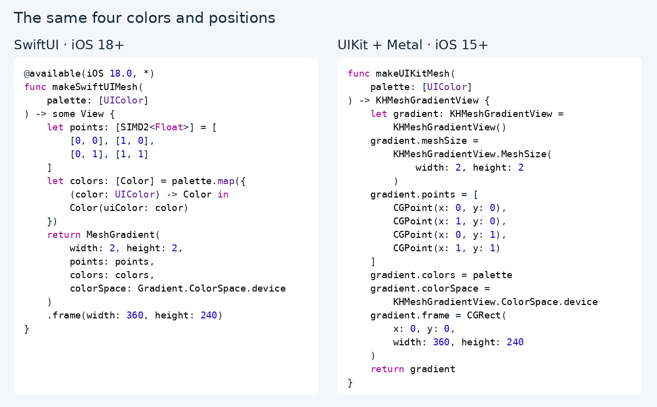
Open the selectable code comparison, or download the complete Swift examples. Both functions explicitly accept palette: [UIColor], with four colors in row-major order; call them with MeshExamples.corners. The comparison page keeps two columns on a wide screen and stacks them on a phone.
For the nine-point example, the UIKit configuration is:
import KHMeshGradient
import UIKit

func makeUIKitRainbow() -> KHMeshGradientView {
	let gradient: KHMeshGradientView = KHMeshGradientView()
	gradient.meshSize = KHMeshGradientView.MeshSize(width: 3, height: 3)
	gradient.points = MeshExamples.grid.map({ (point: SIMD2<Float>) -> CGPoint in
		CGPoint(x: CGFloat(point.x), y: CGFloat(point.y))
	})
	gradient.colors = MeshExamples.rainbow
	gradient.colorSpace = KHMeshGradientView.ColorSpace.device
	return gradient
}
The function returns a configured view. Add it to your UIView hierarchy and assign its frame in layoutSubviews(). meshSize is the library's integer grid type, KHMeshGradientView.MeshSize; it is not a CGSize.
The corresponding controls line up like this:
| SwiftUI | KHMeshGradientView |
|---|---|
width:, height: |
meshSize |
points: |
points |
bezierPoints: |
bezierPoints |
colors: |
colors or resolvedColors |
background: |
meshBackgroundColor |
smoothsColors: |
smoothsColors |
colorSpace: |
colorSpace |
The color-space names should not imply pixel identity. Our .perceptual uses Oklab as an independent approximation. Our additional .linear option uses linear-light sRGB. The gallery's device-color comparisons explicitly select .device on both sides. The library currently outputs 8-bit sRGB, rather than wide-gamut or HDR textures.
From curves to Metal triangles
Our view's backing layer is a custom CAMetalLayer. On the CPU, I turn each patch's four boundary curves into a bicubic position control net with 16 controls. Our construction is a Coons surface: blend opposing boundaries, then subtract their bilinear corner blend so the corner contribution is not counted twice.
The GPU then evaluates the resulting position surface using cubic Bernstein weights:
float4 bernstein(float t) {
	float s = 1.0 - t;
	return float4(s*s*s, 3*s*s*t, 3*s*t*t, t*t*t);
}
For one patch, the evaluation is conceptually:
float2 evaluatePosition(float2 uv, device const float4 *positionNet) {
	float4 bu = bernstein(uv.x);
	float4 bv = bernstein(uv.y);
	float2 position = float2(0);

	for (uint y = 0; y < 4; ++y) {
		for (uint x = 0; x < 4; ++x) {
			position += positionNet[y * 4 + x].xy * bu[x] * bv[y];
		}
	}
	return position;
}
uv is a float2 patch coordinate; positionNet points to that patch's 16 float4 controls in a Metal device buffer. This function uses bernstein defined above. This is an explanatory excerpt: the complete Metal shader indexes each patch's controls, emits clip-space positions, and passes the local UV coordinate to the fragment shader.
We draw an indexed grid of triangles for each patch. If a patch has n subdivisions along each axis, it has n × n cells and 2 × n² triangles. The same index grid can be reused for every patch with that density.
The triangles approximate the curved position surface. They are not the input's colored vertices, and they do not need to be as dense as the output's pixels.
Calculate color per pixel
The first implementation calculated color at the tessellated vertices and let the GPU linearly interpolate it across each triangle. It looked reasonable at high density, but lowering the geometry resolution damaged both shape and color.
The current shader calculates the cubic color surface in the fragment shader. Geometry density now controls the approximation of position and UV; it no longer determines how often we evaluate color. Position/UV errors can still move color features, so this does not make the image completely independent of geometry.
For teaching purposes, color evaluation can be written using the same Bernstein basis:
float4 evaluateColor(float2 uv, device const float4 *colorNet) {
	float4 bu = bernstein(uv.x);
	float4 bv = bernstein(uv.y);
	float4 color = float4(0);
	for (uint y = 0; y < 4; ++y) {
		for (uint x = 0; x < 4; ++x) {
			color += colorNet[y * 4 + x] * bu[x] * bv[y];
		}
	}
	return color;
}
Here colorNet points to 16 derived float4 color controls, not a copy of the position net. The CPU derives the smooth color controls from neighboring colors and handles alpha using premultiplied values.
The shipping shader rearranges the polynomial to reduce arithmetic. It stores one axis in power-basis coefficients and evaluates it with nested fused multiply-add operations:
float4 evaluateFirstColorColumn(float2 uv, device const float4 *net) {
	return fma(
		fma(fma(net[12], uv.y, net[8]), uv.y, net[4]),
		uv.y, net[0]
	);
}
net points to 16 float4 coefficients in the rearranged representation; it is not the Bernstein colorNet from the previous example. The shader calculates the other three columns the same way, then blends those columns with the Bernstein weights along u. Keeping that axis in Bernstein form limits cancellation. Ordinary opaque device-color meshes use packed half-precision coefficients and an RGB-only specialized pipeline. Transparency, other color spaces, and values beyond half range retain float precision; Intel Catalyst also uses the float path.
A straight four-corner patch can therefore display a smooth cubic color field using only two position triangles. Adding triangles just to sample that color field would waste work.
How much geometry does SwiftUI use?
Apple's public documentation describes tessellated Bézier patches. To understand the density choice, I also inspected local RenderBox binaries from iOS 18.2 and 26.5 Simulator and probed buffer construction during actual iOS 26.5 Simulator rendering.
In that inspected implementation, density depends on curvature and rendering scale, rounded to a power of two. A larger view or stronger curve can require more subdivisions. The generated grid is uniform across the retained patches of a mesh; the evidence did not show a separate recursively refined quadtree for every patch. The inspected shader evaluates cubic color in the fragment stage.
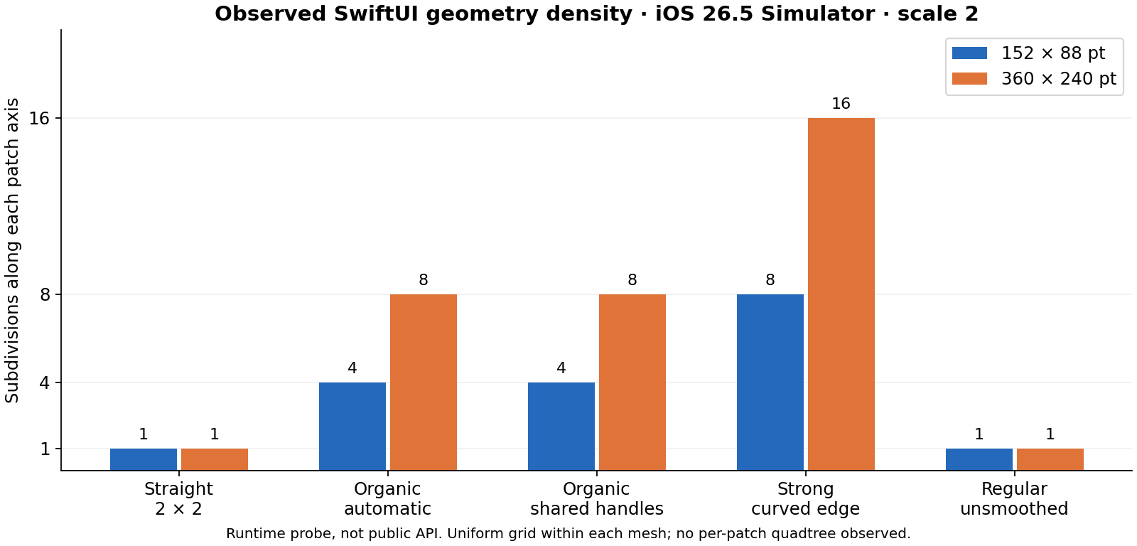
| SwiftUI fixture | 152 × 88 pt | 360 × 240 pt |
|---|---|---|
| Straight four-corner patch, smooth colors | 1 | 1 |
| Organic, automatic handles | 4 | 8 |
| Organic, explicit shared handles | 4 | 8 |
| Strong curved boundary | 8 | 16 |
| Regular grid, unsmoothed colors | 1 | 1 |
Both sizes used scale 2. These are runtime observations from a particular framework version, not public API guarantees. SwiftUI exposes no subdivision knob. Our investigation notes and probe summaries preserve the evidence. The shipping library does not call private framework APIs or include Apple's implementation.
Our adaptive geometry policy
Our independent policy estimates screen-space curvature using second differences of the position control net. It includes pure curvature in each axis and mixed curvature across the patch. The mixed term matters: a surface can have straight boundary curves and still have a nonlinear interior.
The selector increases a uniform power-of-two density until its position-error bound meets a target, or reaches a work limit. In simplified form:
bound = conservative second-derivative bound in framebuffer pixels
n = 1
while bound > target × n² and n < 128:
    n *= 2
reduce n if the mesh would exceed 65,536 cells
The real bound includes the pure and mixed derivative magnitudes. This is our policy, not a reproduction of RenderBox's private arithmetic. All patches in one mesh share a density so their shared boundaries agree; different views can choose different densities.
let gradient: KHMeshGradientView = MeshExamples.makeUIKitRainbow()
gradient.subdivisions = 0           // Adaptive, the default.
gradient.maximumGeometryError = 0.5 // Target deviation in framebuffer pixels.
gradient.debugMode = KHMeshGradientView.DebugMode.tessellation

// Or force a fixed grid for investigation:
gradient.subdivisions = 8
The 128-segment and 65,536-cell caps can override the error target for extreme inputs. The target concerns geometry; it does not guarantee a maximum color difference or SwiftUI parity.
Here are actual exported Metal images for a straight patch and a strongly curved boundary. Each column uses the indicated density; adaptive selection uses the current default policy:
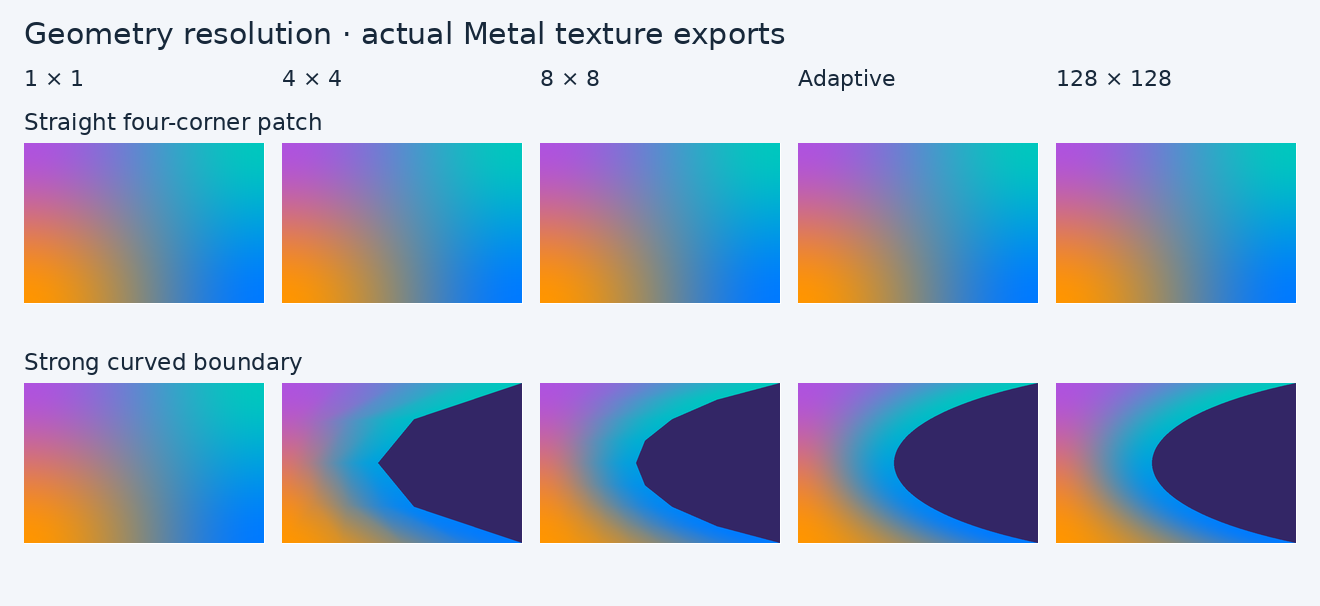
The straight patch needs little geometry. The strongly curved example shows why choosing one low number for everything fails. More detail helps a curved boundary follow its intended shape, but multiplying density everywhere makes the GPU do unnecessary work elsewhere.
Across 15 fixtures at 720 × 480 pixels, adaptive output differs from our own 128-segment reference by 0.016 of an 8-bit channel value on average. That small mean is not a per-pixel guarantee: shifting a high-contrast edge across a pixel can still produce a large local difference. The dense reference is a convergence comparison for our renderer, not proof that it matches SwiftUI.
Continually moving meshes
A lava-lamp effect can evaluate positions from time. For SwiftUI, TimelineView with an AnimationTimelineSchedule provides a time-driven update context:
// Inside a SwiftUI View, available on iOS 18+:
TimelineView(AnimationTimelineSchedule(), content: { (context: TimelineViewDefaultContext) in
	let t: Double = context.date.timeIntervalSinceReferenceDate
	let center: SIMD2<Float> = SIMD2<Float>(
		0.5 + 0.18 * Float(sin(t * 0.7)),
		0.5 + 0.18 * Float(cos(t * 0.9))
	)

	MeshGradient(
		width: 3,
		height: 3,
		points: [
			[0, 0],   [0.5, 0], [1, 0],
			[0, 0.5], center,   [1, 0.5],
			[0, 1],   [0.5, 1], [1, 1]
		],
		colors: MeshExamples.rainbow.map({ (color: UIColor) -> Color in
			Color(uiColor: color)
		}),
		colorSpace: Gradient.ColorSpace.device
	)
})
The calculation uses time, rather than adding a fixed distance on every callback. It therefore follows the same path if the actual refresh cadence changes. TimelineView does not promise a fixed refresh rate.
For a simple repeating UIKit pulse, ordinary animation blocks can animate both the positions and palette:
// This creates the required 3 × 3 grid before accessing its center at index 4.
let gradient: KHMeshGradientView = MeshExamples.makeUIKitRainbow()
UIView.animate(
	withDuration: 4,
	delay: 0,
	options: [
		UIView.AnimationOptions.autoreverse,
		UIView.AnimationOptions.repeat,
		UIView.AnimationOptions.curveEaseInOut
	],
	animations: {
		gradient.points[4] = CGPoint(x: 0.68, y: 0.32)
		gradient.colors[4] = MeshExamples.pink
	},
	completion: nil
)
This UIKit pulse is a different motion path from the sinusoidal SwiftUI example. For a fair performance comparison, our benchmark drives both renderers with the same time-based positions instead.
Our backing layer exposes custom animatable values. Core Animation interpolates those values, and rendering uses the presentation geometry rather than jumping directly to the model's final values. UIViewPropertyAnimator also supports pausing, scrubbing, resuming, and reversing the mesh animation. Its integration uses public Core Animation hooks, though the UIKit action-registration behavior it relies on is undocumented and needs runtime regression testing.
As an animation bends the patches, our geometry selector runs against the current presentation shape and framebuffer size. In the measured 60-view workload, most meshes used 16 subdivisions and some used 32; in the larger-cell workload, they used 32. Density is therefore a response to the changing shape and size, not a fixed “quality level” selected once at initialization. Those counts are observations from the benchmark, not a frame-by-frame trace of every view's choices.
Static meshes keep their last image and submit no recurring GPU work. Dirty views share command buffers, and compatible drawable sizes can share render passes with up to eight independent color targets. Each view still has its own native Metal layer and output texture. Distinct palettes are drawn separately inside the batch; we are not rendering one identical gradient and reusing its image everywhere.
During continuous animation there is always something to redraw. Smooth, slow motion can look good at 60 Hz, while 120 Hz offers finer temporal sampling at a higher sustained workload. Suspend a covered or offscreen animation explicitly when its work is unnecessary.
Do the two renderers look the same?
Here are independently rendered outputs with identical positions, explicit handles where supplied, resolved colors, interpolation settings, dimensions, and appearance:
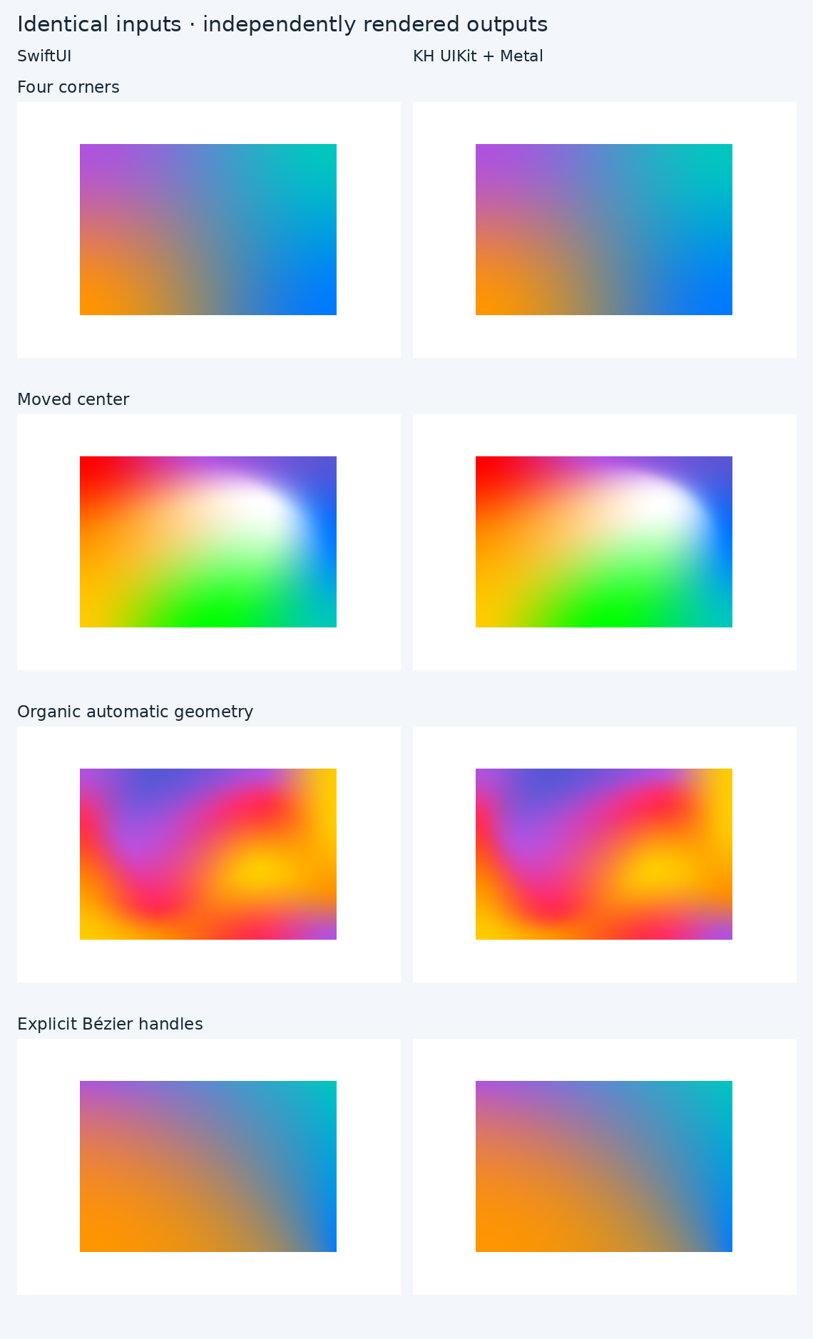
They are close for some inputs and visibly different for others. The organic automatic geometry is a useful example: our inferred handles do not exactly reproduce Apple's. In our preserved geometry experiment, giving both renderers the same explicit handles reduced the small organic fixture's mean RGB difference from about 2.25 to 0.84 channel values out of 255, using that experiment's dense KH reference.
Increasing our subdivisions eventually converges on our surface. It cannot repair a disagreement about what that surface should be. Color-control construction, perceptual interpolation, antialiasing, precision, and dithering can also differ. The article's ordinary gallery was captured on iOS 26.5 Simulator; the geometry-resolution matrix was captured on the physical iPad. SwiftUI reference images use ImageRenderer, and KH images use actual offscreen Metal textures. These quality comparisons are separate from the onscreen performance trials.
What did it cost on a real device?
The current comparison uses an M1 iPad Pro running iPadOS 18.6, with a requested 120 Hz cadence. Each renderer/workload has three fresh-process Release runs, alternating renderer order. Every view has its own distinct palette and independently phased moving geometry; both renderers receive matching inputs.
The meshes are 4 × 4 input grids. The smaller-view workload has 60 cells at 152 × 88 points each. The larger-view workload has 15 cells at 320 × 200 points each. Both use scale 2. The trials stayed at nominal thermal state with Low Power Mode off and all views visible.
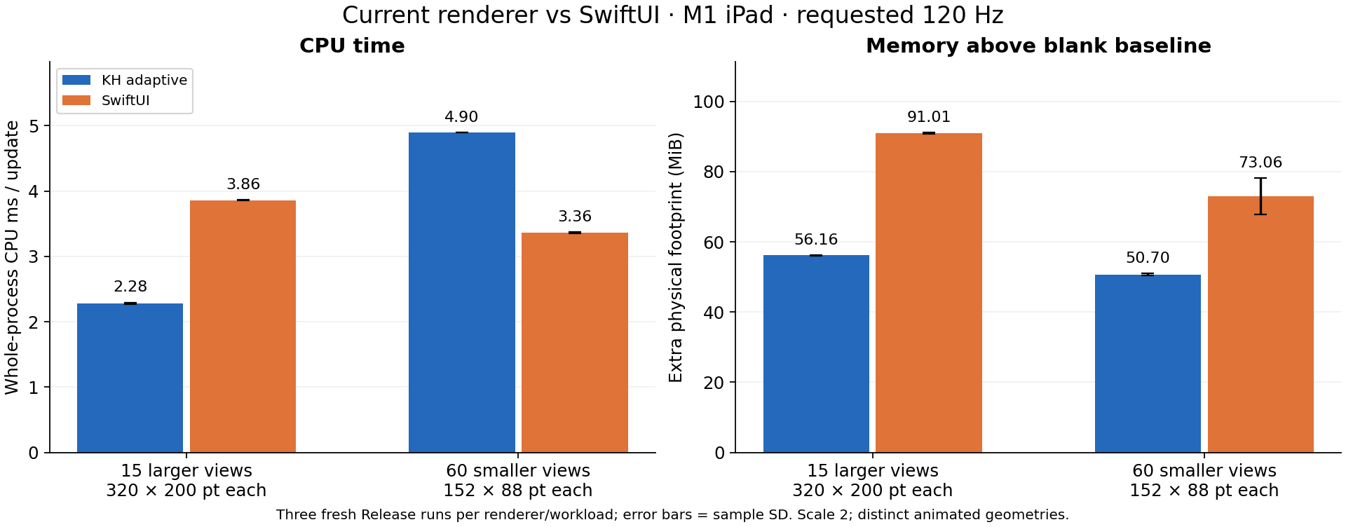
| Workload | KH CPU ms/update | SwiftUI CPU ms/update | KH extra MiB | SwiftUI extra MiB |
|---|---|---|---|---|
| 60 smaller views | 4.90 | 3.36 | 50.70 | 73.06 |
| 15 larger views | 2.28 | 3.86 | 56.16 | 91.01 |
CPU here means whole-process consumed CPU time per update, not main-thread latency. Memory means physical footprint above a fresh blank baseline, not an isolated texture allocation or a universal per-view cost. The compositor is outside these measurements.
SwiftUI uses less CPU in the 60-small-view case. Our renderer uses less CPU in the 15-large-view case and less additional memory in both. A smaller count of larger views is not automatically a cheaper workload: pixel area, CPU submission cost, shared resources, and geometry all matter.
KH's measured presentation rate is approximately 119.93 frames per second per view in both workloads. SwiftUI's callbacks run at about 119.31 and 119.81 updates per second, respectively. Callback frequency is not direct proof of SwiftUI's presented frame rate. CPU and GPU work can overlap, so their durations should not be added together to manufacture a frame time.
GPU work
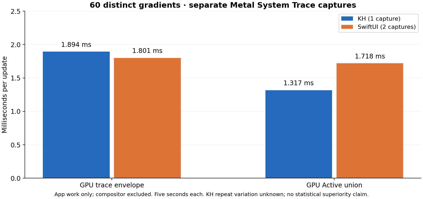
I also captured separate Metal System Trace profiles of the current 60-view scene:
| Metric, 60 distinct views | KH | SwiftUI |
|---|---|---|
| App GPU trace envelope, ms/update | 1.894 | 1.801 |
| GPU Active union, ms/update | 1.317 | 1.718 |
| Vertex Active, ms/update | 0.323 | 0.267 |
| Fragment Active, ms/update | 1.214 | 1.453 |
| Successful five-second profiles | 1 | 2 |
The envelope measures the interval around the observed app GPU stages. Active union measures the time during which at least one observed stage is active. Vertex and fragment activity overlap, so those stage values do not add up to the union. Both renderers submit one app command buffer per update in these captures.
These captures exclude compositor work. Further trace exports failed on unrelated system-daemon timeline errors, so KH's trace repeat variation is unknown. I would not turn this small profile set into a claim that one renderer is universally faster. The separate unprofiled KH diagnostics have three runs, but their command-buffer start/end boundaries differ from the trace envelope; the report keeps them separate.
What adaptive geometry changed
The earlier renderer always used 48 subdivisions and evaluated colors at vertices. For the same 60 distinct animated inputs, the current adaptive, per-fragment implementation changes the measured costs like this:
| Metric | Earlier fixed 48 | Current adaptive |
|---|---|---|
| KH GPU command-buffer envelope, ms/update | 6.42 | 1.85 |
| Extra app physical footprint, MiB | 68.42 | 50.70 |
| Gradient triangles/update | 2,488,320 | about 318,000 |
| Whole-process CPU ms/update | 4.48 | 4.90 |
This reduces the measured GPU interval by about 71%, extra memory by 26%, and triangle count by 87%. The CPU cost rises about 9%. Adaptive selection takes CPU work; it is worthwhile here because it removes much more GPU work. These before/after numbers measure the combined changes, not an isolated experiment on one optimization.
The historical density sweep also shows why quality needs to be measured alongside speed. At fixed 96 subdivisions, KH's reported presentation rate dropped to about 49.9 Hz even while update callbacks averaged about 99.7 Hz. That was the earlier vertex-color implementation, not today's default. It illustrates why counting display-link callbacks alone can miss rendering backpressure.
The current tests animate positions with fixed per-view palettes. They do not establish the sustained thermal cost of a fullscreen lava lamp, performance on every older device, or the extra CPU cost of rebuilding color coefficients for a new palette every frame. Both renderers have convincing headroom for these tested workloads; the actual app still needs measurement at its intended size and animation style.
Try it
KHMeshGradient is a Swift Package Manager library with a basic comparison app, public rendering diagnostics, mesh-debug modes, and support for native UIKit animations. It targets iOS 15 and Mac Catalyst 15; runtime tests currently cover iOS 18.2 and 26.5 Simulator and a physical iPad on iPadOS 18.6. Pre-iOS-18 runtime behavior remains unverified. The source is available under MIT or Apache 2.0, at your option.
The full measurement report includes raw trial JSON, CSV tables, pixel metrics, and capture hashes. The figure provenance records the source files used for this article's graphics.